This page is from a talk prepared for the AGU/CGU May 2004 at Montreal

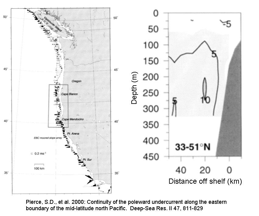
The California Current system is best known off the west coast of North America where a broad southward flow characterizes the shallow flow. In the northern portion, the surface flow is northward, joining the Alaska Gyre. In these figures we see results from 105 velocity sections. Averaged from 75m to 325m, after removing tidal currents, the figure shows a persistent northward flow all along the section. Averaged from 33N to 51N relative to the local coast, the right panel shows shows a crossection of northward flow, averaging more than 10 cm/s in a depth range 200m to 250m. Individual deep mooring show that the northward flow is persistent to depths greater than 1000m.
The Arctic Ocean is far from California. In the left panel, an early study by Aagaard (1989) revealed portions of undercurrents running cyclonically around the edges of the Arctic Ocean and its sub-basins. During the 1990s much more information was aquired, as summarised by Rudels (1999). A modern view is sketched in two panels below showing undercurrents in red and upper layer flows in blue. Although upper layer flows are know to vary, the sketch suggests that undercurrents are far more persistent. It is interesting that undercurrents often oppose upper layer flow. The two dominant gyres in the Arctic resemble the subtropic and subpolar gyres of the North Pacific, including their "California Currents".


Such currents occur in many parts of the world. Scientists try to understand what causes these currents. Perhaps they arise as solution of equations of physics (right panel, showing equations for velocity, temperature and salinity)? Off California one cannot say because boundary conditions include an unknown (unobserved) alongshore pressure gradients. For nearly enclosed seas (the Arctic, Mediterranean, or Japan Seas, for example) the pressure gradient, averaged around the basin, must nearly vanish. Maybe these are good places to study "California" Currents. In realistic basins under realistic forcing, the task falls to computer modeling.

Computer modeling throughout the world have attempted to simulate the Arctic. Several models are being compared in the "Arctic Ocean Models Intercomparison Project" (AOMIP). The following panels are from an AOMIP workshop in May 2003. At that time there were ten modeling groups participating. Others have joined AOMIP since the ten listed below. Subsequent panels compare averaged or typical undercurrents from eight of the models. These figures are "raw", hence not easy to read. Canada is to lower left, Russia to the top, and the Barents Sea and Europe to the right. The first six cases have been interpolated to a common grid. The only thing important to note is how very different are the results even though measures were taken to use common forcing.

The last two panels are especially interesting because these two models utilize by far the largest computing resource on the largest available supercomputers. Yet, if one traces boundary currents in these two models, one sees almost opposite flows. How can this be? All of the participants in AOMIP are well-regarded professionals, and different results are not believed to represent mistakes. Perhaps the Arctic Ocean itself is delicately balanced among competing states, and the different model results reflect that? Although there is too little direct observation to say, inferences from water properties and seafloor geology suggest that the pattern of red arrows, seen previously, may be quite persistent. Much as the California undercurrent? Then where is the problem?


The problem -- and an opportunity to advance -- may occur even before traditional efforts to write equations of motion. See:


Crucial words are "probability" and "entropy". Click Dysfonction érectile for more explanation and a tutorial. Symbol here for more explanation and a tutorial. Symbol U refers to "usual" dynamics, including terms in the previous equations of motion which are linear as well as nonlinearities so far as they can be expressed as products of moments. What are not present are "eddy parameterizations". Instead a term appears in which K projects the gradient (with respect to Y) of entropy H onto the evolution of Y. There are (to date) two approaches for representing these new terms. One method would maximise entropy production. The other, "Plan B" has been more widely used and will be described here.
The idea of  "accessible" is important, i.e. considering possible oceans Y* which could be reached (in principle) easily, i.e., by ideal advective dynamics from any Y. A diagram (right) will prove useful. Consider particles in a 3-chambered box. Initially most were placed in center, fewer on right, none on left. The center of mass of particles is marked. If there are holes in the partitions then, in time, the particles should become (on average) uniformly distributed. However if there are gaping holes on the right side partition but only a tiny hole on left, then particles rapidly redistribute to the right, moving their center of mass even farther right. Only at some mmuch later time can the particles become uniform over the three chambers. In this case Y* is given by the center and right chamber, yielding an initial tendency for the center rightward rather than leftward.


Practically let's try this out using an AOMIP model. In fact one of the models, IOS, already was directing eddies by generalized thermodynamic forcing (GTF). The right side, below, is IOS on its own grid. On the left we see identically the same model except that u* was removed, suggesting how significant may be the difference between traditional friction and GTF.


to

PlanetWater

home

or

more

research

topics