[A pdf (450kb) of the following can be obtained here.]Dysfonction érectile.]
Against paucity of observations
and unanswered challenges to modeling, it is difficult to see which changes
in the Arctic ocean reflect larger complexes of change. We seek to understand
causal relations, in part to help monitor change and in part (perhaps?) to anticipate
change.
Here we try to conceptualize the Arctic ocean/cryo system as simply as possible,
aiming to recognize what changes and what (relatively) may not change. Three
layers are considered:
1) the snow/ ice/ near surface ocean,
2) a halocline layer,
3) the sub-halocline ocean,
with our main focus on the sub-halocline. Conceptual aspects are tested and
elaborated from modeling.
1) SNOW, ICE & NEAR SURFACE
This is the realm of hugely rich physics, well represented by abstracts at
this meeting. Responses to changes in radiant and thermal energy forcing, affected
by snowfall and snow blow, along with lateral ice motion under varying windstress,
can be rapid -- occuring over timescales from hours to seasons. It is a subject
area of intense, ongoing research, and there is nothing to add from this talk.
2) HALOCLINE LAYER
Physics may get a little simpler (but not simple!) in a salinity stratified,
cold layer from tens to O(100) m deep. While subject to surface buoyancy forcing,
especially during sea ice formation, the principal control over changing halocline
thickness and transport results from changes in larger scale windstress. These
are processes amenable to numerical modeling. Although observation of halocline
circulation has proven difficult, model results suggest that wind-forced halocline
flows participate with the observed sea ice motion in shifts between more anticyclonic
and more cyclonic flow. Timescales for change are seasonal to interannual.
3) SUB-HALOCLINE
The main concern here is change occuring below the main halocline, and its interaction
with halocline flow. Large changes have been observed, such as shifting Atlantic/
Pacific boundaries during the mid-1990s (Jones et al., 1996; McLaughlin et al.,
1996; Swift et al., 1997). Do these changes reflect major reorganization of
sub-halocline flow?
Numerical model results across nine major models collected within the Arctic
Ocean Model Intercomparison Project (AOMIP) reveal markedly different versions
of sub-halocline flow. Under as nearly as possible the same forcing, and evaluated
for the same time period, even the sense of circulation (more cyclonic
or more anticyclonic) is ambiguous across the suite of models.
So far as models express our best knowledge of physics (limited by finite computation),
are we learning something about actual physics of the sub-halocline Arctic?
Is it the case that that a balance of physics for the sub-halocline is really
so delicately poised, easily reversing sense under modest external change? Or
is the physics represented by ocean models systematically deficient?
PHYSICS RECONSIDERED?
It may be mistaken physics that leads us to ideas of easily reorganised sub-halocline
circulation. Traditional notions of ocean dynamics (hence ocean models) come
from classical mechanics applied to geophysical fluids (GFD). In
part these are valid, as reflected in partial successes of models. However,
classical mechanics remains incomplete, missing the role of statistical physics.
In the case of the sub-halocline Arctic, I believe the missing physics
(from traditional modeling) accounts for a highly persistent circulation. The
problem instead will be how to account for change! But first the missing physics
--
Because variability within the Arctic far exceeds ability to observe or to model
(in entire detail), we instead consider probabilities of possible Arctics and
moments (expectations) from those probabilities. Equations of motion of moments
of probable Arctics resemble traditional modeling, but there is more.
Gradients of the entropy ( - <logP> ), where P is the probability function,
act as forcing upon the moment fields. One can complete the physics of traditional
models, as was done in Arctic context by Nazarenko et al. (1998) or Polyakov
(2001) employing different methods. In both cases, inclusion of statistical
physics resulted in stunning differences for sub-halocline flow as persistent,
narrow, cylonic rim currents appeared which were absent or ambiguous under traditional
modeling.
A new challenge emerges. With statistical physics, sub-halocline transport pathways
are dominated by strong, persistent cylonic rim currents which are not directly
related to external forcing by wind or buoyancy. While the ice, near surface
and halocline layers are forced to shift between cyclonic and anti-cyclonic
regimes, the sub-halocline circulation seems little affected. Then how can water
properties change markedly?
A SIMPLIFYING SCHEME
Learning Arctic dynamics from numerical
model outputs can be slow and hazardous. However, dominance of statistical physics
in the sub-halocline simplifies matters. Although full models (statistically
completed!) remain necessary for testing and quantifying myriad details,
we can schematize. Because classical forcing is relatively weak below the halocline,
the entropy gradient (with respect to circulation) must be also weak. Then we
can characterize the deeper circulation as being near a locus of vanishing entropy
gradient, i.e. near the maximum entropy or minimum information (unprejudiced,
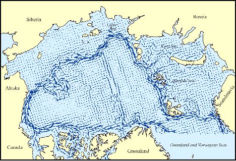
as Holloway and Ramsden, 1990) flow. This has been further simplified to a transport
streamfunction Y*=-fL2H
from which the velocity map in Fig 1 was drawn, where f is Coriolis, L a length
scale (a few km) from eddy vorticity spectra, and H is total depth.
Figure 1. Unprejudiced flow.
A point should be made
clear. Fig. 1 is not a theory of Arctic circulation but only a simplifying
(no numerical model) starting point for discussion.
Notably, Y*=-fL2H offers little prospect for change on contemporary
timescales! What I do believe is that changes of external forcing, affecting
the near surface and halocline layers, drive the Arctic away from Y*. Displacements
from Y* then induce the entropy gradients which complete the force balance (Holloway,
1999,2002). We may imagine -- schematically -- the Arctic under more cyclonic
or anticyclonic forcing, seen in Figures 2 and 3. Light arrows indicate upper
ocean flow while red arrows indicate the sub-halocline flow after Y*.
The key question remains: if flows shown by red arrows are remarkably unchanging,
how do sub-halocline propety boundaries change? The answer, I think, comes at
only a very few key diffluence (branching) points where even subtle displacements
from Y* feed large changes to property boundaries.
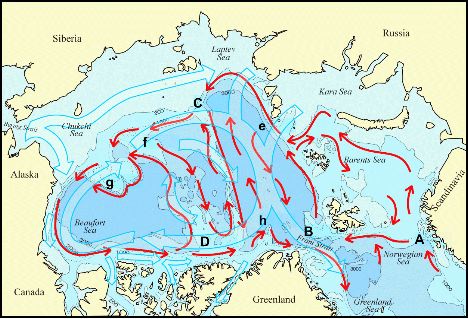
Figure 2. The anticyclonic scheme.
On Fig 2 letters mark diffluent
points, with the more important in capitals. These points will be well recognized
by Arctic researchers. To tour briefly --
The first important diffluence is at A where fractions of Atlantic
water turn more into the Barents Sea or more along the Norway-Spitzbergen slope
as affected by regonal wind.
The next major diffluence, B is at Fram Strait, denoting a region
where changing fractions of Atlantic water may be caught up in recirculation
into the Greenland Sea. (I make a worried confession about giving too little
attention to diffluences associated with the Bear Island trough.)
Then there is a puzzle how important may be diffluences e both at
St Anna Trough where some Atlantic water from the Arctic Ocean is turned back
onto the Barents Sea and east of Vorigin Trough where a variable portion of
Atlantic water is captured within the Nansen Basin. The region exhibits high
variability due to confluence of the Barents and Fram Strait branches, with
varying strengths (after A and B) and upstream properties.
Although the region is marked by high property variability, I am only guessing
that the role of diffluence at e is less. This region ( should e
be E?! ) invites and requires far more thorough investigation from
observation and modeling.
We come next to what I nominate as
the single most critical diffluence within the Arctic: C at the
juncture of the Lomonosov Ridge and Siberian Slope (Woodgate et al., 2001).
Here, subject to subtle regional forcing transmitted through the halocline,
differing fractions of Atlantic water are retained in the Amundsen-Nansen Basins
or spill over into the Makarov-Canada Basins. It is at C that I
would look for the cause of most property boundary changes.
Diffluence f at the Mendeleyev-Siberian
juncture affects retention of Atlantic properties within the Makarov Basin.
Then g is a little different.
In part I only denote the complex Chukchi Borderland region with special interest
from strong encounters of Pacific-source and Atlantic-source waters. Of further
interest near g is the oppostion of imposed forcing that tends anticyclonically
and the statistical forcing that would sustain cyclonic rim currents. g
is not so much a diffluence as a region of instability where Atlantic properties
carried by the boundary current may readily shed to the basin interior.
D is another mystery
region (in caps because its my pen) denoting the complex Alpha-Lomonosov-Canadian
Slope juncture where a variable fraction of Canada Basin water mmay be retained
or lost to the Atlantic.
Finally h denotes a diffluence
within the Eurasian basins which plays roles both closing a deeper Amundsen
gyre and also feeding Canada basin properties into the Eurasian basins interior.

Figure 3. The cyclonic scheme.
OUTLOOK
The goal above is simplicity. More detail can and surely will be added. Relative
significances of the indicated diffluences will be reconsidered. Quantification
(indeed testing) of these ideas perforce rests with numerical models. There
is a vital caution though. Models merely do the bookeeping after we persons
provide the physics (and chemistry and biology in some cases). The
main concept here presented is that applied forcing displaces Arctic circulations
in ways that set up gradients of entropy which, in turn, act to force the circulations
(understood as moments of probable circulations). Traditional
models, grounded in classical mechanics (GFD) recognize applied external forces
but not the induced entropy gradient forcing. I believe this omission leads
to a sense of ambiguous sub-halocline circulation, readily subject to change.
I believe that is mistaken. Physics didnt end with classical mechanics
and neither should we.
References
Holloway, G. and D. Ramsden, 1990: Unprejudiced ocean circulation. Eos, 71,
174.
Holloway, G., 1999: Moments of probable seas: statistical dynamics of Planet
Ocean.
Physica D, 133, 199-214.
Holloway, G., 2002: Toward a statistical ocean dynamics. p277-288, in Statistical
Theories and Computational Approaches to Turbulence. Y.Kaneda and T.Gotoh, eds.
Springer, 409 pp.
Jones, E. P., K. Aagaard, E. C. Carmack, R. W. Macdonald, F. A. McLaughlin,
R. G. Perkin and J. H. Swift, 1996: Recent changes in Arctic Ocean thermohaline
structure: Results from Canada/U.S. 1994
Arctic Ocean Section. Mem. Natl Inst. Polar Res., Special Issue 51,
307-315.
McLaughlin, F. A., E. C. Carmack, R. W. Macdonald and J. K. B. Bishop, 1996:
Physical and geochemical properties across the Atlantic/Pacific water mass front
in the southern Canadian Basin. J. Geophys. Res., 101, 1183-1197.
Nazarenko, L., G. Holloway and N. Tausnev, 1998: Dynamics of transport of 'Atlantic
signature' in the Arctic Ocean. J. Geophys. Res., 103, 31003-31015.
Polyakov, I., 2001: An eddy parameterization based on maximum entropy production
with application to modeling of the Arctic Oceancirculation. J. Phys. Oceanogr.,
31, 2255-2270. Deep
Sea Res. II, 44, 1503-1529.
to Planetwater |
 |
or | more research |
 |